Tag Archives: feature vectors

Nudging discoveries along the innovation path

Decorative photograph of a Welsh hill
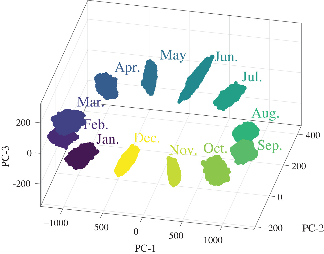
The path from a discovery to a successful innovation is often tortuous and many good ideas fall by the wayside.  I have periodically reported on progress along the path for our novel technique for extracting feature vectors from maps of strain data [see ‘Recognizing strain‘ on October 28th, 2015] and its application to validating models of structures by comparing predicted and measured data [see ‘Million to one‘ on November 21st, 2018], and to tracking damage in composite materials [see ‘Spatio-temporal damage maps‘ on May 6th, 2020] as well as in metallic aircraft structures [see ‘Out of the valley of death into a hype cycle‘ on February 24th 2021].  As industrial case studies, we have deployed the technology for validation of predictions of structural behaviour of a prototype aircraft cockpit [see ‘The blind leading the blind‘ on May 27th, 2020] as part of the MOTIVATE project and for damage detection during a wing test as part of the DIMES project.  As a result of the experience gained in these case studies, we recently published an enhanced version of our technique for extracting feature vectors that allows us to handle data from irregularly shaped objects or data sets with gaps in them [Christian et al, 2021].  Now, as part of the Smarter Testing project [see ‘Jigsaw puzzling without a picture‘ on October 27th, 2021] and in collaboration with Dassault Systemes, we have developed a web-based widget that implements the enhanced technique for extracting feature vectors and compares datasets from computational models and physical models.  The THEON web-based widget is available together with a video demonstration of its use and a user manual.  We supplied some exemplar datasets based on our work in structural mechanics as supplementary material associated with our publication; however, it is applicable across a wide range of fields including earth sciences, as we demonstrated in our recent work on El Niño events [see ‘From strain measurements to assessing El Niño events‘ on March 17th, 2021].  We feel that we have taken some significant steps along the innovation path which will lead to adoption of our technique by a wider community; but only time will tell whether this technology survives or falls by the wayside despite our efforts to keep it on track.

Bibliography

Christian WJR, Dvurecenska K, Amjad K, Pierce J, Przybyla C & Patterson EA, Real-time quantification of damage in structural materials during mechanical testing, Royal Society Open Science, 7:191407, 2020.

Christian WJ, Dean AD, Dvurecenska K, Middleton CA, Patterson EA. Comparing full-field data from structural components with complicated geometries. Royal Society open science. 8(9):210916, 2021

Dvurecenska K, Graham S, Patelli E & Patterson EA, A probabilistic metric for the validation of computational models, Royal Society Open Science, 5:1180687, 2018.

Middleton CA, Weihrauch M, Christian WJR, Greene RJ & Patterson EA, Detection and tracking of cracks based on thermoelastic stress analysis, R. Soc. Open Sci. 7:200823, 2020.

Wang W, Mottershead JE, Patki A, Patterson EA, Construction of shape features for the representation of full-field displacement/strain data, Applied Mechanics and Materials, 24-25:365-370, 2010.

From strain measurements to assessing El Niño events

Figure 11 from RSOS 201086One of the exciting aspects of leading a university research group is that you can never be quite sure where the research is going next.  We published a nice example of this unpredictability last week in Royal Society Open Science in a paper called ‘Transformation of measurement uncertainties into low-dimensional feature space‘ [1].  While the title is an accurate description of the contents, it does not give much away and certainly does not reveal that we proposed a new method for assessing the occurrence of El Niño events.  For some time we have been working with massive datasets of measurements from arrays of sensors and representing them by fitting polynomials in a process known as image decomposition [see ‘Recognising strain‘ on October 28th, 2015]. The relatively small number of coefficients from these polynomials can be collated into a feature vector which facilitates comparison with other datasets [see for example, ‘Out of the valley of death into a hype cycle‘ on February 24th, 2021].  Our recent paper provides a solution to the issue of representing the measurement uncertainty in the same space as the feature vector which is roughly what we set out to do.  We demonstrated our new method for representing the measurement uncertainty by calibrating and validating a computational model of a simple beam in bending using data from an earlier study in a EU-funded project called VANESSA [2] — so no surprises there.  However, then my co-author and PhD student, Antonis Alexiadis went looking for other interesting datasets with which to demonstrate the new method.  He found a set of spatially-varying uncertainties associated with a metamodel of soil moisture in a river basin in China [3] and global oceanographic temperature fields collected monthly over 11 years from 2002 to 2012 [4].  We used the latter set of data to develop a new technique for assessing the occurrence of El-Niño events in the Pacific Ocean.  Our technique is based on global ocean dynamics rather than on the small region in the Pacific Ocean which is usually used and has the added advantages of providing a confidence level on the assessment as well as enabling straightforward comparisons of predictions and measurements.  The comparison of predictions and measurements is a recurring theme in our current research but I did not expect it to lead into ocean dynamics.

Image is Figure 11 from [1] showing convex hulls fitted to the cloud of points representing the uncertainty intervals for the ocean temperature measurements for each month in 2002 using only the three most significant principal components . The lack of overlap between hulls can be interpreted as implying a significant difference in the temperature between months.

References:

[1] Alexiadis, A. and Ferson, S. and  Patterson, E.A., , 2021. Transformation of measurement uncertainties into low-dimensional feature vector space. Royal Society Open Science, 8(3): 201086.

[2] Lampeas G, Pasialis V, Lin X, Patterson EA. 2015.  On the validation of solid mechanics models using optical measurements and data decomposition. Simulation Modelling Practice and Theory 52, 92-107.

[3] Kang J, Jin R, Li X, Zhang Y. 2017, Block Kriging with measurement errors: a case study of the spatial prediction of soil moisture in the middle reaches of Heihe River Basin. IEEE Geoscience and Remote Sensing Letters, 14, 87-91.

[4] Gaillard F, Reynaud T, Thierry V, Kolodziejczyk N, von Schuckmann K. 2016. In situ-based reanalysis of the global ocean temperature and salinity with ISAS: variability of the heat content and steric height. J. Climate. 29, 1305-1323.

Alleviating industrial uncertainty

Want to know how to assess the quality of predictions of structural deformation from a computational model and how to diagnose the causes of differences between measurements and predictions?  The MOTIVATE project has the answers; that might seem like an over-assertive claim but read on and make your own judgment.  Eighteen months ago, I reported on a new method for quantifying the uncertainty present in measurements of deformation made in an industrial environment [see ‘Industrial uncertainty’ on December 12th, 2018] that we were trialling on a 1 m square panel of an aircraft fuselage.  Recently, we have used the measurement uncertainty we found to make judgments about the quality of predictions from computer models of the panel under compressive loading.  The top graphic shows the outside surface of the panel (left) with a speckle pattern to allow measurements of its deformation using digital image correlation (DIC) [see ‘256 shades of grey‘ on January 22, 2014 for a brief explanation of DIC]; and the inside surface (right) with stringers and ribs.  The bottom graphic shows our results for two load cases: a 50 kN compression (top row) and a 50 kN compression and 1 degree of torsion (bottom row).  The left column shows the out-of-plane deformation measured using a stereoscopic DIC system and the middle row shows the corresponding predictions from a computational model using finite element analysis [see ‘Did cubism inspire engineering analysis?’ on January 25th, 2017].  We have described these deformation fields in a reduced form using feature vectors by applying image decomposition [see ‘Recognizing strain’ on October 28th, 2015 for a brief explanation of image decomposition].  The elements of the feature vectors are known as shape descriptors and corresponding pairs of them, from the measurements and predictions, are plotted in the graphs on the right in the bottom graphic for each load case.  If the predictions were in perfect agreement with measurements then all of the points on these graphs would lie on the line equality [y=x] which is the solid line on each graph.  However, perfect agreement is unobtainable because there will always be uncertainty present; so, the question arises, how much deviation from the solid line is acceptable?  One answer is that the deviation should be less than the uncertainty present in the measurements that we evaluated with our new method and is shown by the dashed lines.  Hence, when all of the points fall inside the dashed lines then the predictions are at least as good as the measurements.  If some points lie outside of the dashed lines, then we can look at the form of the corresponding shape descriptors to start diagnosing why we have significant differences between our model and experiment.  The forms of these outlying shape descriptors are shown as insets on the plots.  However, busy, or non-technical decision-makers are often not interested in this level of detailed analysis and instead just want to know how good the predictions are.  To answer this question, we have implemented a validation metric (VM) that we developed [see ‘Million to one’ on November 21st, 2018] which allows us to state the probability that the predictions and measurements are from the same population given the known uncertainty in the measurements – these probabilities are shown in the black boxes superimposed on the graphs.

These novel methods create a toolbox for alleviating uncertainty about predictions of structural behaviour in industrial contexts.  Please get in touch if you want more information in order to test these tools yourself.

The MOTIVATE project has received funding from the Clean Sky 2 Joint Undertaking under the European Union’s Horizon 2020 research and innovation programme under grant agreement No. 754660 and the Swiss State Secretariat for Education, Research and Innovation under contract number 17.00064.

The opinions expressed in this blog post reflect only the author’s view and the Clean Sky 2 Joint Undertaking is not responsible for any use that may be made of the information it contains.