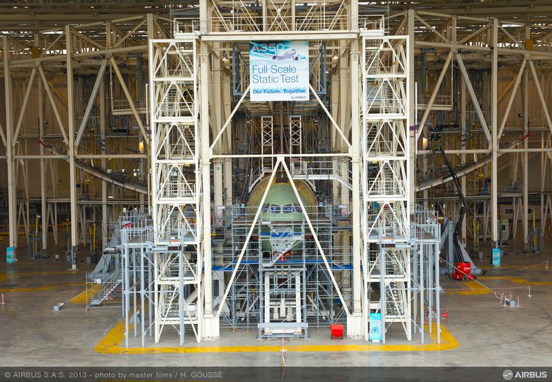
A350 XWB passes Maximum Wing Bending test
Research sometimes feels like putting together a jigsaw puzzle without the picture or being sure you have all of the pieces. The pieces we are trying to fit together at the moment are (i) image decomposition of strain fields [see ‘Recognising strain’ on October 28th 2015] that allows fields containing millions of data values to be represented by a feature vector with only tens of elements which is useful for comparing maps or fields of predictions from a computational model with measurements made in the real-world; (ii) evaluation of the variation in measurement uncertainty over a field of view of measured displacements or strains in a large structure [see ‘Industrial uncertainty’ on December 12th 2018] which provides information about the quality of the measurements; and (iii) a probabilistic validation metric that provides a measure of how well predictions from a computational model represent measurements made in the real world [see ‘Million to one’ on November 21st 2018]. We have found some of the missing pieces of the jigsaw, for example we have established how to represent the distribution of measurement uncertainty in the feature vector domain [see ‘From strain measurements to assessing El Niño events’ on March 17th 2021] so that it can be used to assess the significance of differences between measurements and predictions represented by their feature vectors – this connects (i) and (ii) together. Very recently we have demonstrated a generic technique for performing image decomposition of irregularly shaped fields of data or data fields with holes [see Christian et al, 2021] which extends the applicability of our method for comparing measurements and predictions to real-world objects rather than idealised shapes. This allows (i) to be used in industrial applications but we still have to work out how to connect this to the probabilistic metric in (iii) while also incorporating spatially-varying uncertainty. These techniques can be used in a wide range of applications, as demonstrated in our recent work on El Niño events [see Alexiadis et al, 2021], because, by treating all fields of data as images, the techniques are agnostic about the source and format of the data. However, at the moment, our main focus is on their application to ground tests on aircraft structures as part of the Smarter Testing project in collaboration with Airbus, Centre for Modelling & Simulation, Dassault Systèmes, GOM UK Ltd, and the National Physical Laboratory with funding from the Aerospace Technology Institute. Together we are working towards digital continuity across virtual and physical testing of aircraft structures to provide live data fusion and enable condition-led inspections, test control and validation of computational models. We anticipate these advances will reduce time and costs for physical tests and accelerate the development of new designs of aircraft that will contribute to global sustainability targets (the aerospace industry has committed to reduce CO2 emissions to 50% of 2005 levels by 2050). The Smarter Testing project has an ambitious goal which reveals that our pieces of the jigsaw puzzle belong to a small section of a much larger one.
For more on the Smarter Testing project see:
References
Alexiadis A, Ferson S, Patterson EA. Transformation of measurement uncertainties into low-dimensional feature vector space. Royal Society open science. 8(3):201086, 2021.
Christian WJ, Dean AD, Dvurecenska K, Middleton CA, Patterson EA. Comparing full-field data from structural components with complicated geometries. Royal Society open science. 8(9):210916, 2021.