 This is a question that both my undergraduate students and a group of taught post-graduates have struggled with this month. In thermodynamics, my undergraduate students were estimating absolute zero in degrees Celsius using a simple manometer and a digital thermometer (this is an experiment from my MOOC: Energy – Thermodynamics in Everyday Life). They needed to know how many times to repeat the experiment in order to determine whether their result was significantly different to the theoretical value: -273 degrees Celsius [see my post entitled ‘Arbitrary zero‘ on February 13th, 2013 and ‘Beyond zero‘ the following week]. Meanwhile, the post-graduate students were measuring the strain distribution in a metal plate with a central hole that was loaded in tension. They needed to know how many times to repeat the experiment to obtain meaningful results that would allow a decision to be made about the validity of their computer simulation of the experiment [see my post entitled ‘Getting smarter‘ on June 21st, 2017].
The simple answer is six repeats are needed if you want 98% confidence in the conclusion and you are happy to accept that the margin of error and the standard deviation of your sample are equal. The latter implies that error bars of the mean plus and minus one standard deviation are also 98% confidence limits, which is often convenient. Not surprisingly, only a few undergraduate students figured that out and repeated their experiment six times; and the post-graduates pooled their data to give them a large enough sample size.
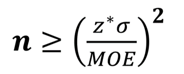
The justification for this answer lies in an equation that relates the number in a sample, n to the margin of error, MOE, the standard deviation of the sample, σ, and the shape of the normal distribution described by the z-score or z-statistic, z*:  The margin of error, MOE, is the maximum expected difference between the true value of a parameter and the sample estimate of the parameter which is usually the mean of the sample. While the standard deviation, σ, describes the difference between the data values in the sample and the mean value of the sample, μ. If we don’t know one of these quantities then we can simplify the equation by assuming that they are equal; and then n ≥ (z*)².
The z-statistic is the number of standard deviations from the mean that a data value lies, i.e, the distance from the mean in a Normal distribution, as shown in the graphic [for more on the Normal distribution, see my post entitled ‘Uncertainty about Bayesian methods‘ on June 7th, 2017]. We can specify its value so that the interval defined by its positive and negative value contains 98% of the distribution. The values of z for 90%, 95%, 98% and 99% are shown in the table in the graphic with corresponding values of (z*)², which are equivalent to minimum values of the sample size, n (the number of repeats).
Confidence limits are defined as:  but when n = z², this simplifies to μ ± σ. So, with a sample size of six (6 = n ≥ z² for 98% confidence) we can state with 98% confidence that there is no significant difference between our mean estimate and the theoretical value of absolute zero when that difference is less than the standard deviation of our six estimates.
BTW – the apparatus for the thermodynamics experiments costs less than £10. The instruction sheet is available here – it is not quite an Everyday Engineering Example but the experiment is designed to be performed in your kitchen rather than a laboratory.
 I wrote this short annual report in anticipation of being on vacation this week. However, as my editor commented, it is ‘a bit of a non-blog’ and so I have written a second post for today that will be published a few minutes later.

 or CC BY-SA 3.0 (http://creativecommons.org/licenses/by-sa/3.0)], via Wikimedia Commons")

