 Last June, I wrote about representing five-dimensional data using a three-dimensional stack of transparent cubes containing fairy lights whose brightness varied with time and also using feature vectors in which the data are compressed into a relatively short string of numbers [see ‘Fairy lights and decomposing multi-dimensional datasets’ on June 14th, 2023]. After many iterations, we have finally had an article published describing our method of orthogonally decomposing multi-dimensional data arrays using Chebyshev polynomials. In this context, orthogonal means that components of the resultant feature vector are statistically independent of one another. The decomposition process consists of fitting a particular form of polynomials, or equations, to the data by varying the coefficients in the polynomials. The values of the coefficients become the components of the feature vector. This is what we do when we fit a straight line of the form y=mx+c to set of values of x and y and the coefficients are m and c which can be used to compare data from different sources, instead of the datasets themselves. For example, x and y might be the daily sales of ice cream and the daily average temperature with different datasets relating to different locations. Of course, it is much harder for data that is non-linear and varying with w, x, y and z, such as the intensity of light in the stack of transparent cubes with fairy lights inside. In our article, we did not use fairy lights or icecream sales, instead we compared the measurements and predictions in two case studies: the internal stresses in a simple composite specimen and the time-varying surface displacements of a vibrating panel.
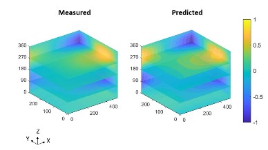
The image shows the normalised out-of-plane displacements as the colour as a function of time in the z-direction for the surface of a panel represented by the xy-plane.
Source:
Amjad KH, Christian WJ, Dvurecenska KS, Mollenhauer D, Przybyla CP, Patterson EA. Quantitative Comparisons of Volumetric Datasets from Experiments and Computational Models. IEEE Access. 11: 123401-123417, 2023.